TL;DR:
This blog focuses on the topic of Domain Adaptation, specifically in the unsupervised case and classification task. However, it does not cover semi-domain adaptation at this time. Domain Adaptation is a common challenge in machine learning that arises when there is a distribution mismatch between the training and testing data.
This blog post is inspired by the Stanford CS330 Deep Multi-Task & Meta Learning lecture series, specifically Lecture 13 and 14. I watch the lectures, then conducting codes and experiments for a more practical learning.
The blog series will be divided into three parts: Covariate Shift, Adversarial Training and CycleGAN.In each part, I will provide both theoretical explanations and practical code examples for understanding and implementing these concepts.
This is the first technical blog I have written for learning and sharing purposes, and mistakes may occur. I hope to receive any feedback. Let’s learn together!
1. What is Domain Adaptation?
Definition
Domain adaptation a common issue when the characteristics or distributions of the training and testing datasets are different.
In domain adaptation, the source domain is where we have examples with labels that we can use to train our model (usually train set). The target domain is where we want our model to work well, even if we don’t have many or any labeled examples from that domain (usually validation set). The goal is to use what we learned from the source domain to make our model perform better in the target domain.
Domain Adaptation is the task of adapting models across domains. This is motivated by the challenge where the test and training datasets fall from different data distributions due to some factor. Domain adaptation aims to build machine learning models that can be generalized into a target domain and dealing with the discrepancy across domain distributions. Source: paperwithcode.com
Example 1: let’s consider a competition where you train a model on a dataset of colored images (MNIST-M). However, during evaluation, you are provided with black and white images (MNIST). Similarly, you may encounter a situation where you are given a grayscale image, but you need to build a model for color images.

Image 1 - Training dataset: MNIST-M; MNIST-M is created by combining MNIST digits with the patches randomly extracted from color photos of BSDS500 as their background. It contains 59,001 training and 90,001 test images.
Example 2: imagine you develop a model to classify different types of white blood cells using data from one hospital. However, when you try to use the same model in another hospital, the imaging techniques and conditions may differ, resulting in a decrease in performance. This situation becomes more complex when dealing with three datasets: Raabin, BCCD, and LISC, which may originate from various countries, hospitals, and equipment.

Some samples of the WBCs in Raabin-WBC, LISC, and BCCD datasets; Source
The problem setting of limited data has gained significant attention and importance in recent times. This blog post is inspired by the Stanford CS330 Deep Multi-Task & Meta Learning lecture series, specifically Lecture 13 and 14. I followed a similar structure to the lectures and mathematical explaination. Then I conducted an experiment using the MNIST-M and MNIST datasets.
This series of blog will have 3 part: This blog series will be divided into three parts:
- Part 1: Covariate Shift (including theoretical background and code)
- Part 2: Adversarial Training in Domain Adaptation (including theoretical background and code)
- Part 3: Cycle-GAN on Domain Translation (including theoretical background and, hopefully, code if I can complete it on time)
Notation
Let’s get used to some notation (read it slowly!):
- We have a data sample x and it label y.
- Model hypothesis: \( f_{\theta}(x) \) . Where \( f_{\theta}\) , can be any model, linear regression, SVM…or any Deep Learning model.
- Loss on 1 sample: \( \mathcal{L}(f_{\theta}(x), y) \) . Which measure distance between model output and it ground truth label.
- Distribution of \(\color{teal}{\text{train set (or Source dataset)}}\) : \(\color{teal}{P_{S}(x, y)} \)
- Distribution of \(\color{magenta}{\text{test set (or Target dataset)}}\) : \(\color{magenta}{P_{T}(x, y)} \)
We then use expectation to calculate the loss function for the train and test sets:
-
Loss (or error) function on \(\color{teal}{\text{train set}}\) : \( \epsilon_{\color{teal}{S}}(f_{\theta})= E_{\color{teal}{P_{S}(x, y)}} [\mathcal{L}(f_{\theta}(x), y )] \) This loss funciton average the errors or losses of our model’s predictions over all the training samples.
-
Loss (or error) function on \(\color{magenta}{\text{test set}}\) \( \epsilon_{\color{magenta}{S}}(f_{\theta})= E_{\color{magenta}{P_{T}(x, y)}} [\mathcal{L}(f_{\theta}(x), y )].\) .Similarly, we calculate the loss on the test set to evaluate how well our model generalizes to unseen data.
General Assumption of Domain Adatation
- The source and target domain are only differ in domain of the function. Which i.e: \(\color{teal}{P_{S}(y|x)} \) = \(\color{magenta}{P_{T}(y|x)} \)
- There exist a single hypothesis with low error.
Source: Stanford CS330 Deep Multi-Task & Meta Learning - Domain Adaptation l 2022 I Lecture 13
2. Covariate Shift Problem
Problem setting
Covariate shift refers to a specific problem in domain adaptation, where the distribution of the training data differs from the distribution of the testing data, but with additional asssumption about the distribution of domain and target dataset.
Additional assumption: the support (range of values) of the source domain is larger than or equal to the support of the target domain. this means that the source domain covers a wider range of possible input features compared to the target domain.
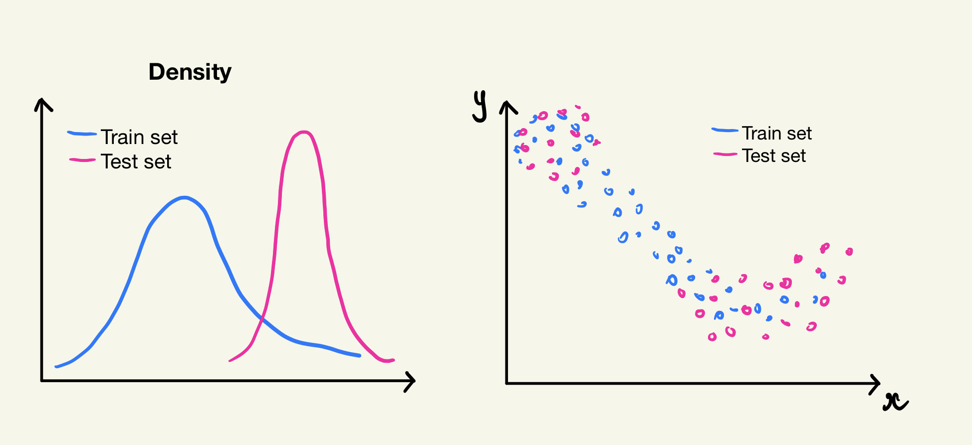
Covariate Shift occur when a model have distribution of train set different from its test set, but the range of distribution of train set are larger than test set’s
Solution
Our Objective : Minimize \( \epsilon_{\color{magenta}{T}}(f_{\theta}) \) under the assumption the distribution of train set and test set are not similar.
💡 A simple solution is: re-weight the samples in the training set based on their likelihood of being representative of the test set (reweighting score), which mean assigning higher weights to samples that are more likely to be representative of the test. Doing so, we are assigning a higher prioritize for samples that are having more predicting ability on test set.
Mathematical ground
For those who care about the “WHY”, let’s move to the this section. For those who are more interested in the “HOW”, you can skip ahead to the Implementation section.
Let do some math together. Don’t worries, we can do it!
Firstly, we recall the formular of expectation for a function:
- Expectation of a function:
\[E[g(Z)] = \int f(z) \cdot g(z) \, dz \]
- \(g(z) \) : function of Random Variable \(X\)
- \(E[g(Z)] \) : the expectation of the function
- \(f(z) \) : is the probability density function (PDF) of the random variable. The integral is taken over the entire range of possible values of \( Z\)
Secondly, let go back to the objective and break down the mathematical expressions of the objectives:
\[\epsilon_{\color{magenta}{T}}(f_{\theta}) = E_{\color{magenta}{P_{T}(x, y)}}[\mathcal{L}(f_{\theta}(x), y )] =\int \color{magenta}{P_{T}(x, y)} \mathcal{L}(f_{\theta}(x), y ) dx dy \\ \it{\color{gray}{ \text{#in this step, we expand the formular of expectation in the form of intergal}} }\] \[ =\int \color{magenta}{P_{T}(x, y)} \frac{\color{teal}{P_{S}(x, y)}} {\color{teal}{P_{S}(x, y)}} \mathcal{L}(f_{\theta}(x), y) dx dy \] \[= \int {\color{teal}{P_{S}(x, y)}} \frac{\color{magenta}{P_{T}(x, y)}} {\color{teal}{P_{S}(x, y)}} \mathcal{L}(f_{\theta}(x), y) dx dy \\ \it{ \color{gray}{ \text{# in these 2 rows, we adding 1 which is also}} \frac{\color{teal}{P_{S}(x, y)}} {\color{teal}{P_{S}(x, y)}} \color{gray}{\text{and then modify the position}} } \] \[ \it{ \color{gray}{ \text{#to understand next lines, we need to revisit the expectation formular for a function E[g(x)] above: } \\ \int \color{brown}{f(z)} \cdot \color{pink}{g(z)}\, dz = E_{Z}[g(z)] } , \color{gray}{ \text{similarly, let change the color code of the line above, we have } \\ \int \color{brown}{P_{S}(x, y)} \cdot \color{pink}{ \frac{{P_{T}(x, y)}}{{P_{S}(x, y)}} \mathcal{L}(f_{\theta}(x), y) }\, dx dy } \\ \color{gray}{\text{Here we have pdf: } \color{brown}{f(z) = P_{S}(x, y)} \text{ and a function of X and Y are : } \color{pink}{g(x) = \frac{{P_{T}(x, y)}}{{P_{S}(x, y)}} \mathcal{L}(f_{\theta}(x), y) }\ } } \] \[ = E_{\color{teal}{P_{S}(x, y)}} [ \frac{\color{magenta}{P_{T}(x, y)}} {\color{teal}{P_{S}(x, y)}} \mathcal{L}(f_{\theta}(x), y) ] \\ \] \[ = E_{\color{teal}{P_{S}(x, y)}} [ \frac{\color{magenta}{P_{T}(x | y) P_{T}(y)}} {\color{teal}{P_{S}(x| y) P_{S}(y)}} \mathcal{L}(f_{\theta}(x), y) ] \\ \it{\color{gray}{ \text{using Bayes Rules}}} \] \[ = E_{\color{teal}{P_{S}(x, y)}} [ \frac{\color{magenta}{P_{T}(x)}} {\color{teal}{P_{S}(x)}} \mathcal{L}(f_{\theta}(x), y)] \\ \it{\color{gray}{ \text{we can reduce term above by assumption of Domain Adaption is } \color{teal}{P_{S}(x | y)} = \color{magenta}{P_{T}(x | y)} } } \]
❓ How to compute: \( E_{\color{teal}{P_{S}(x, y)}} [ \frac{\color{magenta}{P_{T}(x)}} {\color{teal}{P_{S}(x)}} \mathcal{L}(f_{\theta}(x), y)] \) ?
💡 We up-weight on samples on train set with high likelihood on target distribution (hight
\( \color{teal}{P_{S}(x)} \)
) and low likelihood on source distribution (low
\( \color{magenta}{P_{T}(x)} \)
). This is called Important Sampling (Importance Sampling is technique in Numerical Methods (a subject I almost failed in school 😅)
❓ Then, next question, how to Estimate this Proportion \(\frac{\color{magenta}{P_{T}(x)}} {\color{teal}{P_{S}(x)}} \)
💡To estimate this proportion, we can train a domain classifier to distinguish between the source and target domains. A domain classifier is a model that is trained to classify samples into their respective domains, typically the source and target domains. When the domain classifier outputs a prediction of 0, it means that the sample is classified as belonging to the source domain. A prediction of 1 indicates that the sample is classified as belonging to the target domain.
Algorithm
\[ - Step 1: \text{Train a Domain Classifier} : cls(\text{source} | x) \\ - Step 2: \text{Reweight the Loss function with} \frac{1-cls(\text{source} | x)}{cls(\text{source} | x)} \\ (Note: \color{magenta}{p(\text{target} | X_{i})} = 1 - \color{teal}{p(\text{source} | X_{i})}) \]
Proof of why we can perform Importance Sampling in the problem setting using a Domain Classifier:
- We have \[ \color{magenta}{p_{T}(X) = P(X | \text{domain = T}) = \frac{{p(\text{domain = T} | X) \cdot p(X)}}{{p(\text{domain = target})}}} \] \[ \color{teal}{p_{S}(X) = P(X | \text{domain = S}) = \frac{{p(\text{domain = S} | X) \cdot p(X)}}{{p(\text{domain = source})}}} \]
- Then
\[ \frac{{\color{magenta}{p_{T}(x)}}}{{\color{teal}{p_{S}(X)}}} = \frac{{\color{magenta}{p(X | \text{domain = T})}}}{{\color{teal}{p(X | \text{domain = S})}}} \] \[= \color{magenta}{\frac{{p(\text{domain = T} | X) \cdot p(X)}}{{p(\text{domain = target})}}} \cdot \color{teal}{\frac{{p(\text{domain = source})}}{{p(\text{domain = S} | X) \cdot p(X)}}} \] \[ = \color{magenta}{\frac{{p(\text{domain = T} | X)}}{{p(\text{domain = target})}}} \cdot \color{teal}{\frac{{p(\text{domain = source})}}{{p(\text{domain = S} | X)}}} \] \[ = \frac{{\color{magenta}{p(\text{domain = T} | X)}}}{{\color{teal}{p(\text{domain = S} | X)}}} \cdot \frac{{\color{teal}{p(\text{domain = source})}}}{{\color{magenta}{p(\text{domain = target})}}} \] \[ = \frac{{\color{magenta}{p(\text{domain = T} | X)}}}{{\color{teal}{p(\text{domain = S} | X)}}} \cdot \text{constant} \]
Implementation
Model
So, to simplify, we will just need:
- Model 1 - a domain classifer: This model classifies whether a given sample of data is coming from the source domain or the target domain. An output value of 1 indicates that the given sample is predicted to be from the source domain, otherwise it is predicted as target domain.
We then use the probability output of the classifier as a reweighting score for each sample to “reweight” the loss function for the label classifier.
\[ \text{Reweight the Loss function with} = \frac{ \color{teal}{1-{cls(\text{source} | x)}} }{ \color{teal}{ cls(\text{source} | x)} } \]\( \color{teal}{1-{cls(\text{source| x)}}} \) : represents the probability or confidence that a given sample “x” belongs to the target domain.
- Model 2 - a label classifier: This model performs classification and incorporates a reweight score by multiplying it in the second step mentioned above using ReweightLossfunction
Experiment Details
We will apply the solution on mnist dataset with 2 settings:
- Setting 1 MNIST-M -> MNIST: MNIST-M as source domain, MNIST as target domain
- Setting 2 MNIST -> MNIST-M: MNIST as source domain, MNIST-M as target domain (code bellow are for setting 1, please check for both setting)
Example github link:
Model 1- Domain Classifier
- Let create a simple CNN for the Domain Classifer
import torch
import torch.nn as nn

class DomainClassifier(nn.Module):
    def __init__(self):
        super(DomainClassifier, self).__init__()

        self.feature_extractor = nn.Sequential(
            nn.Conv2d(3, 64, kernel_size=5),
            nn.BatchNorm2d(64),
            nn.MaxPool2d(2),
            nn.ReLU(True),
            nn.Conv2d(64, 50, kernel_size=5),
            nn.BatchNorm2d(50),
            nn.Dropout2d(),
            nn.MaxPool2d(2),
            nn.ReLU(True)
        )

        self.classifier = nn.Sequential(
            nn.Linear(50 * 4 * 4, 100),
            nn.BatchNorm1d(100),
            nn.ReLU(True),
            nn.Dropout2d(),
            nn.Linear(100, 100),
            nn.BatchNorm1d(100),
            nn.ReLU(True),
            nn.Linear(100, 2),
            nn.Softmax(dim=1)
        )

    def forward(self, input_img):
        feature = self.feature_extractor(input_img)
        feature = feature.view(feature.size(0), -1)  # Flatten the feature tensor
        domain_prob = self.classifier(feature)
        # domain_prob = torch.softmax(domain_output, dim=1)
        return domain_prob
- We create the
TargetSourceDatsetto train the Domain Classifier
from torch.utils.data import Dataset, DataLoader

class TargetSourceDataset(Dataset):

    def __init__(self, target_dataset, source_dataset):
        self.target_dataset = target_dataset
        self.source_dataset = source_dataset

    def __len__(self):
        return len(self.target_dataset) + len(self.source_dataset)

    def __getitem__(self, index):
        if index < len(self.target_dataset):
            image, _ = self.target_dataset[index]
            domain_label = 0  # Target domain label
        else:
            source_index = index - len(self.target_dataset)
            image, _ = self.source_dataset[source_index]
            domain_label = 1  # Source domain label

        return image, domain_label

# Create the combined dataset
target_source_dataset = TargetSourceDataset(target_dataloader.dataset, source_dataloader.dataset)
# Create the combined dataloader
target_source_dataloader = DataLoader(target_source_dataset, batch_size=batch_size, shuffle=True)
- Training Domain Classifier:
lr = 1e-4
batch_size = 128
image_size = 28
n_epoch = 2

domain_classifier = DomainClassifier().to(device)
loss = nn.CrossEntropyLoss()
optimizer = torch.optim.Adam(domain_classifier.parameters(), lr=lr)


LOSS_DOMAIN = []
ACC_DOMAIN = []

for epoch in range(n_epoch):
    correct = 0
    total_samples = 0

    len_target_source_dataloader = len(target_source_dataloader)
    for i, (img, label) in enumerate(target_source_dataloader):
        batch_size = len(img)
        input_img = img.to(device)

        label_output = domain_classifier(input_img)
        label_pred = torch.argmax(label_output, dim=1)

        label = label.to(device)

        correct += (label_pred == label).sum().item()
        total_samples += len(label)

        label_acc = 100.0 * correct / total_samples
        _loss = loss(label_output, label)

        ACC_DOMAIN.append(label_acc)
        LOSS_DOMAIN.append(_loss.item())

        optimizer.zero_grad()
        _loss.backward()
        optimizer.step()

        if (i % 100) == 0 and i!= 0:
            print(f'epoch: {epoch+1}, [iter: {i:03d} / all {len_target_source_dataloader}], '
                    f'loss_label: {_loss.item():.4f}, '
                    f'| label acc: {label_acc:.4f}')
We visualize output of the Domain Classifier, after computing the re-weighting score for each sample. As the images plotted, the images that have higher reweights score to the domain output are very similar to the TARGET domain.
Top highest re-weighting score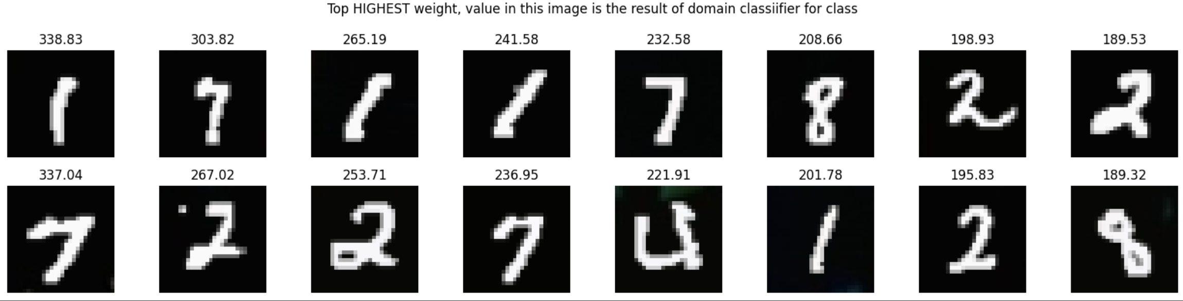
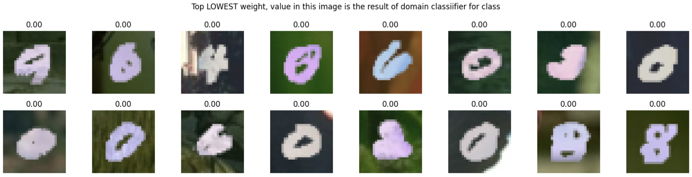
Top lowest re-weighting score
Loss function
We create the loss function as:
class ReweightedCrossEntropyLoss(nn.Module):

    def __init__(self):
        super(ReweightedCrossEntropyLoss, self).__init__()
        self.loss_function = nn.CrossEntropyLoss()

    def forward(self, input, target, domain_output):
        # Calculate the standard CrossEntropyLoss
        loss = self.loss_function(input, target)

        # Calculate the weight as domain_output[:, 0] / domain_output[:, 1]
        weight = domain_output[:, 0] / domain_output[:, 1]

        # Apply the weight factor
        weighted_loss = (weight * loss).mean()
        return weighted_loss
However, the important weight can be blow up if the target domain is large which cause imbalance for model learning. There is several solutions mentions in lecture Covariate Shift (David S. Rosenberg (NYU: CDS))
To address this issue and mitigate the imbalance, we use both clipping and square root transformations in the loss function. Clipping can limit the range of the reweight scores, preventing extreme values from dominating the training process. Applying the square root transformation helps to reduce the disparity between large and small reweight scores, promoting a more balanced influence of different samples on the model’s learning.
Final loss function after modification:
class ReweightedCrossEntropyLoss(nn.Module):
    def __init__(self):
        super(ReweightedCrossEntropyLoss, self).__init__()
        self.loss_function = nn.CrossEntropyLoss(reduction='none')

    def forward(self, input, label, domain_output, threshold, max_value):
        # Calculate the standard CrossEntropyLoss
        loss = self.loss_function(input, label)

        source_prob = domain_output[:, 1]
        target_prob = domain_output[:, 0]
        weights = torch.sqrt(target_prob / (source_prob + 1e-8))  # Add a small epsilon to avoid division by zero

        weights = torch.where(weights < threshold, torch.tensor(threshold), weights)
        weights = torch.where(weights > max_value, torch.tensor(max_value), weights)

        weighted_loss = (weights * loss).mean()

        return weighted_loss
Model 2: Label Classifier
- Label Classifier: a simple and shallow one
class LabelClassifier(nn.Module):
    def __init__(self):
        super(LabelClassifier, self).__init__()

        self.feature_extractor = nn.Sequential(
            nn.Conv2d(3, 16, kernel_size=3),
            nn.ReLU(inplace=True),
            nn.MaxPool2d(2),
            nn.Conv2d(16, 32, kernel_size=3),
            nn.ReLU(inplace=True),
            nn.MaxPool2d(2)
        )

        self.classifier = nn.Sequential(
            nn.Linear(32 * 5 * 5, 100),
            nn.ReLU(inplace=True),
            nn.Linear(100, 10)
        )

    def forward(self, input_img):
        feature = self.feature_extractor(input_img)
        feature = feature.view(feature.size(0), -1)  # Flatten the feature tensor
        output = self.classifier(feature)
        return output
Train the Label Classifier
- We create
CombinedDataset: placedholder for input of the label classifier which would include source images, label of source image, domain label (1 for source and 0 for target)
import torch
import matplotlib.pyplot as plt
from torch.utils.data import DataLoader, Dataset

# Define a custom dataset for the combined data
class CombinedDataset(Dataset):
    def __init__(self, images, labels, domain_outputs):
        self.images = images
        self.labels = labels
        self.domain_outputs = domain_outputs

    def __getitem__(self, index):
        image = self.images[index]
        label = self.labels[index]
        domain_output = self.domain_outputs[index]
        return image, label, domain_output

    def __len__(self):
        return len(self.images)
Run the prediction of Domain Classifier on Source Domain and save result in the CombinedDataset
# Calculate overall accuracy
total_correct = 0
total_samples = 0

domain_classifier.eval()  # Set the model to evaluation mode

domain_outputs = []
source_images_list = []
source_labels_list = []

with torch.no_grad():
    for images, source_labels in source_dataloader:
        input_images = images.to(device)
        labels = torch.ones(images.size(0), dtype=torch.long).to(device)

        domain_output = domain_classifier(input_images)
        _, domain_pred = torch.max(domain_output, 1)

        total_correct += (domain_pred == labels).sum().item()
        total_samples += len(labels)

        # print(100.0 * correct/total)

        domain_outputs.append(domain_output)
        source_images_list.append(input_images)
        source_labels_list.append(source_labels)

# Concatenate the domain outputs, images, and labels
combined_domain_output = torch.cat(domain_outputs, dim=0)
combined_source_images = torch.cat(source_images_list, dim=0)
combined_source_labels = torch.cat(source_labels_list, dim=0)

combined_dataset = CombinedDataset(combined_source_images, combined_source_labels, combined_domain_output)

accuracy = 100.0 * total_correct / total_samples
print(f"Accuracy of domain classifier: {accuracy:.4f}%")

batch_size = 128


combined_dataloader = DataLoader(
    combined_dataset,
    batch_size=batch_size,
    shuffle=True
)
- Train the Label Classifier, the prediction was run on TARGET domain and displayed the accuracy after each epoch; We perform 5 runs and record the average accuracy
thes = 3
max_value = 4


lr = 1e-3
batch_size = 128
image_size = 28
n_epoch = 5


output_accuracies = []
for run_num in range(5) :
    LOSS_LABEL = []
    ACC_LABEL = []

    # Model, Loss, and Optimizer
    label_classifier = LabelClassifier().to(device)
    loss_label = ReweightedCrossEntropyLoss()
    optimizer = optim.Adam(label_classifier.parameters(), lr=lr)

    # Training loop
    input_dataloader = combined_dataloader
    acc_result = []
    for epoch in range(n_epoch):
        correct = 0
        total_samples = 0
        data_iter = iter(input_dataloader)
        for i in range(len(input_dataloader)):
            len_dataloader = len(input_dataloader)
            data_source = next(data_iter)
            img, label, domain_clf_output = data_source
            batch_size = len(img)
            input_img = img.to(device)
            label = label.to(device)
            label_output = label_classifier(input_img)
            label_pred = torch.argmax(label_output, dim=1)
            correct += (label_pred == label).sum().item()
            total_samples += batch_size
            label_acc = 100.0 * correct / total_samples
            with torch.no_grad():
                detached_domain_output = domain_clf_output.detach()
            loss = loss_label(label_output, label, domain_clf_output, thes, max_value)
            ACC_LABEL.append(label_acc)
            LOSS_LABEL.append(loss)
            optimizer.zero_grad()
            loss.backward()
            optimizer.step()
            if (i % 200) == 0 and i != 0:
                print(f'epoch: {epoch+1}, [iter: {i:03d} / all {len_dataloader}], '
                    f'loss label: {loss.item():.4f}, '
                    f'| label acc (SOURCE): {label_acc:.4f}')


        # run on test set after each epochs to monitor result on test set (target set)
        domain_outputs = []
        source_train_images_list = []
        source_train_labels_list = []
        total_correct = 0
        total_samples = 0
        label_classifier.eval()
        for batch_data in target_dataloader:
            train_images, train_labels = batch_data
            batch_size = len(train_labels)
            input_images = train_images.to(device)
            class_label = train_labels.to(device)
            with torch.no_grad():
                pred_output = label_classifier(input_images)
                class_pred = torch.argmax(pred_output, dim=1)
                correct = (class_pred == class_label).sum().item()
                total = len(class_label)
                total_correct += correct
                total_samples += total
        accuracy = 100.0 * total_correct / total_samples
        print(f"Accuracy of label classifier (on TARGET) with reweight loss after epoch {epoch+1}: {accuracy:.4f}%")
        acc_result.append(accuracy)
    output_accuracies.append(accuracy)

    print("Run num: ", run_num, ', '.join([f'{i:.4f}' for i in acc_result]))
    print("------------------------------------------")
    print("\n")


print("-> Accuracies of 5 runs: ", ', '.join([f'{i:.2f}' for i in output_accuracies]))
_acc  = np.array(output_accuracies)
_avg = np.mean(_acc, axis=0)

print(f"-> Average accuracy of 5 runs: {_avg:.2f}")
>>
------------------------------------------


-> Accuracies of 5 runs:  96.87, 97.09, 96.80, 97.31, 96.86
-> Average accuracy of 5 runs: 96.99
Comparision
Now, let compare with Traditional Implementation (without the Domain Classifer) by using the standard CrossEntropyLoss
import torch.optim as optim

# Hyperparameters
lr = 1e-3
batch_size = 128
image_size = 28
n_epoch = 5

output_accuracies = []
for run_num in range(5):
    output = []


    # Model, Loss, and Optimizer
    traditional_label_classifier = LabelClassifier().to(device)
    loss_label_no_dc = nn.CrossEntropyLoss()
    optimizer = optim.Adam(traditional_label_classifier.parameters(), lr=lr)

    # Training loop
    CLASSICAL_LOSS_LABEL = []
    CLASSICAL_ACC_LABEL = []

    for epoch in range(n_epoch):
        correct = 0
        total_samples = 0
        input_dataloader = combined_dataloader
        data_iter = iter(input_dataloader)

        for i in range(len(input_dataloader)):
            len_dataloader = len(input_dataloader)

            data_source = next(data_iter)
            img, label, _= data_source
            batch_size = len(img)
            input_img = img.to(device)
            label = label.to(device)

            label_output = traditional_label_classifier(input_img)
            label_pred = torch.argmax(label_output, dim=1)

            correct += (label_pred == label).sum().item()
            total_samples += len(label)

            label_acc = 100.0 * correct / total_samples
            loss = loss_label_no_dc(label_output, label)

            CLASSICAL_ACC_LABEL.append(label_acc)
            CLASSICAL_LOSS_LABEL.append(loss.item())

            optimizer.zero_grad()
            loss.backward()
            optimizer.step()

            if (i % 200) == 0 and i != 0:
                print(f'epoch: {epoch+1}, [iter: {i:03d} / all {len_dataloader}], '
                      f'loss label: {loss.item():.4f}, '
                      f'| label acc (SOURCE): {label_acc:.4f}')

        # Evaluation on target dataset after each epoch
        domain_outputs = []
        source_train_images_list = []
        source_train_labels_list = []

        total_correct = 0
        total_samples = 0

        traditional_label_classifier.eval()

        for batch_data in target_dataloader:
            train_images, train_labels = batch_data
            batch_size = len(train_labels)

            input_images = train_images.to(device)
            class_label = train_labels.to(device)

            with torch.no_grad():
                pred_output = traditional_label_classifier(input_images)
                class_pred = torch.argmax(pred_output, dim=1)

                correct = (class_pred == class_label).sum().item()
                total = len(class_label)

                total_correct += correct
                total_samples += total

        accuracy = 100.0 * total_correct / total_samples
        print(f"- Accuracy of label classifier (predict on TARGET) after epoch {epoch+1}: {accuracy:.2f}%")
        output.append(accuracy)

    output_accuracies.append(accuracy)

    print('Run number', run_num, '|', ', '.join([f'{i:.2f}' for i in output]))
    print("\n")

print("\n")
print("-> Accuracies of 5 runs: ", ', '.join([f'{i:.2f}' for i in output_accuracies]))
_acc  = np.array(output_accuracies)
_avg = np.mean(_acc, axis=0)

print(f"-> Average accuracy of 5 runs: {_avg:.2f}")
Result:
-> Accuracies of 5 runs:  96.83, 96.09, 96.69, 96.94, 96.79
-> Average accuracy of 5 runs: 96.67
Please check this Github link for the full notebook above:
Result on 2 setting
MNIST-M -> MNIST: MNIST-M as source and
| Accuracy | MNIST-M -> MNIST | MNIST -> mnist-M |
|---|---|---|
| Traditional (average of 5 runs) | 96.67% | 55.31% |
| Covariate - Shift (average of 5 runs) | 96.99% | 57.22% |
Discussion and future parts
Analysis: Before we continue, let’s address a question: \[ \color{red}{\text{Why does the result of Covariate Shift} \\ \text{perform well in the case of } \text{MNIST-M} \rightarrow \text{MNIST} \\ \text{but poorly in the case of MNIST} \rightarrow {MNIST-M?}} \]
Comment: Let’s revisit the assumption of the covariate shift problem setting that is that the support (range of values) of the source domain is larger than or equal to the support of the target domain. We observe that in the MNIST-M (source) -> MNIST (target) case, the model still captures features related to the target set because there are many samples that are similar to the test set (colorized images can generalize to black and white). However, in the MNIST (source) -> MNIST-M (target) case, the source dataset does not cover the domain of the domain set (black and white cannot generalize to colorized images).
In the next blogs, we will explore two other powerful techniques to handle situations where the support of the test set is not within the training set, Domain Adversarial Training and CycleGAN.
According to the table below, we can see that Domain Adversarial Training handles the situation very well in the MNIST -> MNIST-M case. In the covariate shift problem, we focus on mapping the sample space, but with domain adversarial training, we concentrate on the feature space. We aim to find a feature space that is general enough to represent both domains (invariant domain features).
| Accuracy | MNIST-M -> MNIST | MNIST -> mnist-M |
|---|---|---|
| Traditional (average of 5 runs) | 96.67% | 55.31% |
| Covariate - Shift (average of 5 runs) | 96.99% | 57.22% |
| Domain Adversarial Training | 96.61% | 72.08% |
In Part 3, we will delve into a more advanced technique related to GANs, known as CycleGAN, where we generate samples from domain A while incorporating domain information from another domain, B.
Isn’t it interesting? Please Let me know your comment and feedback. See you in the next posts!